Survival Analysis

\[ \renewcommand{\P}{\mathsf{P}} \newcommand{\m}{\mathsf{m}} \newcommand{\p}{\mathsf{p}} \newcommand{\q}{\mathsf{q}} \newcommand{\bb}{\mathsf{b}} \newcommand{\g}{\mathsf{g}} \newcommand{\rr}{\mathsf{r}} \newcommand{\IF}{\mathbb{IF}} \newcommand{\dd}{\mathsf{d}} \newcommand{\Pn}{$\mathsf{P}_n$} \newcommand{\E}{\mathsf{E}} \]

Data considerations

• Similar to when the outcome is binary, survival outcomes should be coded using 0’s and 1’s where 1 indicates the occurrence of an event and 0 otherwise.

• Similar to how we encode censoring variables, we consider the outcome to be degenerate. Meaning that once an observation experiences an outcome, all future outcome variables should also be coded with a 1 (“last-observation-carried-forward”).

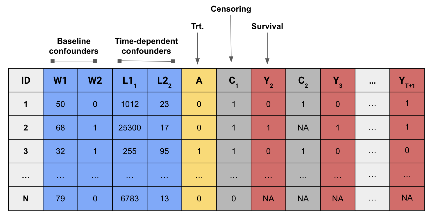
Point-treatment survival problems

Up to this point, we’ve been ignoring that the covid dataset should be treated as a point-treatment survival problem. Let’s re-estimate the effect of the randomized treatment with a survival framework.

• We need to transform the data from long to wide format

• and impute the outcome using last-observation-carried-forward.

Our modified dataset should look like this:

Structure of data with survival outcome and point-treatment. Adapted from Hoffman et al., 2022.

Use the function event_locf() to make sure the outcome variables are correctly recorded.

• Instead of just estimating the effect of treatment on the outcome at the last time point, we can estimate the effect of a treatment on an outcome at all follow-up intervals.

Let’s estimate the effect of the treatment on intubation at each day. To do so, we can use the function lmtp_survival() .

We can now visualize our results using a survival plot.

The main result of an lmtp object can be extracted using the tidy() function from the broom package.

Time-varying treatment

Hoffman et al. (2024) demonstrated the use of modified treatment policies for survival outcomes to assess the effect of delaying invasive mechanical ventilation (IMV) on mortality among patients hospitalized with COVID-19 in New York City during the first COVID-19 wave. A synthetic version of the data used for that analysis has been loaded into R as intubation.

Structure of data with survival outcome and time-varying treatment. Adapted from Hoffman et al., 2022.

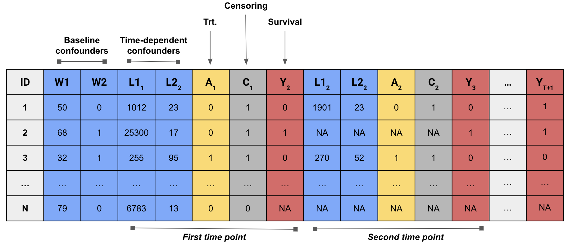
• The data consists of \(n = 2000\) observations hospitalized with COVID-19 and who were followed for \(\tau = 14\) days.

• There are 10 baseline confounders and 4 time-varying confounders.

• The outcome of interest is an indicator for death on day \(t\).

• Observations are subject to loss-to-follow-up due to either hospital discharge or transfer.

Let’s consider the following intervention

\[ \dd_t(a_t, h_t) = \begin{cases} 1 \text{ if } a_t = 2 \text{ and } a_s \leq 1 \forall s < t \\ a_t \text{ otherwise}, \end{cases} \]

where \(A_t\) is a 3-level categorical variable: 0, no supplemental oxygen; 1, non-IMV supplemental oxygen support; 2, IMV.

In words, this function corresponds to an intervention where patients who were naturally observed as receiving IMV on day \(t\) instead had IMV delayed by a day to day \(t+1\). Let’s translate this policy to an R function that we can use with lmtp.

Question: Why might defining an intervention in terms of an MTP instead of a static intervention be more useful to answer a question about the effect of IMV on death among patients hospitalized with COVID-19?

✅ Answer

Intubation may increase the likelihood of mortality through factors separate from COVID (by increasing the likelihood of AKI, for example); however, not intubating a patient who is in respiratory distress may also increase the likelihood of mortality. Thus, some patients do need to be intubated and an intervention that eliminated intubation all together would be non-nonsensical.

We can now estimate the effect of delaying IMV by 1-day on 14-day mortality.

Competing risks

In the context of survival analysis, competing risks refer to events that preclude the occurrence of the primary event of interest. In the previous example, we treated hospital discharge or transfer as censoring events. These events, however, are actually competing risks because we know that if a patients was discharged or transferred out of the ICU on day \(t\) they didn’t die on that day.

Treating competing risks as censoring events involves estimating the effect of an intervention that eliminates the competing event. The identification assumptions for this intervention are stronger than intervention that doesn’t consider eliminating the competing event.

In the presence of competing risks, lmtp can estimate cumulative incidence effects. Cumulative incidence effect can be interpreted as the total effect of treatment operating through pathways that include the competing events. Let’s re-evaluate the effect of a delaying IMV 1-day on 14-day mortality but instead treat discharge or transfer as a competing risk. We first need to modify the data:

• Flip the columns corresponding to discharge or transfer so that a 1 indicates a discharge or transfer occurred
• Impute missing values for discharge and death using last-observation carried forward because they are both deterministic variables once they have occurred (i.e., if a patient died, their probability of discharge or transfer is 0 and vice-versa)

We can now re-estimate the effect of delaying IMV by 1-day. Instead of passing the discharge vector to the cens argument, we pass it to the compete argument.

References

Dı́az, Iván, Katherine L Hoffman, and Nima S Hejazi. 2024. “Causal Survival Analysis Under Competing Risks Using Longitudinal Modified Treatment Policies.” Lifetime Data Analysis 30 (1): 213–36.

Dı́az, Iván, Nicholas Williams, Katherine L Hoffman, and Edward J Schenck. 2023. “Nonparametric Causal Effects Based on Longitudinal Modified Treatment Policies.” Journal of the American Statistical Association 118 (542): 846–57.

Hoffman, Katherine L., Diego Salazar-Barreto, Nicholas Williams, Kara E. Rudolph, and Ivan Diaz. 2024. “Studying Continuous, Time-Varying, and/or Complex Exposures Using Longitudinal Modified Treatment Policies.” https://arxiv.org/abs/2304.09460.

Young, Jessica G, Mats J Stensrud, Eric J Tchetgen Tchetgen, and Miguel A Hernán. 2020. “A Causal Framework for Classical Statistical Estimands in Failure-Time Settings with Competing Events.” Statistics in Medicine 39 (8): 1199–1236.