install.packages("lmtp")The lmtp package
So far, we’ve
Defined a causal estimand for general, hypothetical interventions
Identified that estimand from observational data
Discussed 4 different estimators.
It’s now time to move on to applying this new knowledge to real data examples.
Existing software and lmtp
General software for estimation of causal effects in longitudinal studies is limited:
The
ipwandgfoRmulapackages provide routines for estimating causal effects using inverse probability weighting (IPW) and the parametric g-formula respectively. As we already discussed, however, the validity of these methods requires making unrealistic parametric assumptions.The
ltmleandsurvtmlepackages implement a doubly-robust method for estimating causal effects from longitudinal data, but these packages do not support continuous valued exposures, multiple exposures, interventions that depend on the natural value of the exposure, or stochastic interventions.
In contrast, the lmtp package (software companion to the paper by Dı́az et al. (2023)) can be used to doubly robustly and flexibly estimate point-in-time and longitudinal effects of the general set of interventions that we’ve talked about today.
- lmtp could be your default package for conducting causal analyses in R!
Installation
For this workshop, lmtp has already been installed with webr. However, you can install the package locally on your machine from CRAN with
Alternatively, you can download the developmental version from GitHub with
# install.packages(devtools)
devtools::install_github("nt-williams/lmtp@devel")
Preliminaries
Before we move on to using lmtp, here’s general information that will be applicable across all examples:
Data is passed to estimators through the
dataargument.Data should be in wide format with one column per variable per time point under study (i.e., there should be one column for every variable in \(O\)). Data may be either a
data.frameortibblebut not adata.table.Columns do not have to be in any specific order and the data may contain variables that are not used in estimation.
The names of treatment variables are specified with the
trtargument.The names of censoring variables are specified with the
censargument.The names of baseline covariates are specified with the
baselineargument.The names of time-varying covariates are specified with the
time_varyargument.The
trtargument accepts either a character vector or a list of character vectors.The
censandbaselinearguments accept character vectors.The
time_varyargument accepts a list of character vectors.
Vectors and lists are basic data structures in R. A vector can be thought of as a 1-dimensional collection of homogeneous elements. For example a character vector is a collection of values with the class character.
a_character_vector <- c("this", "is", "a", "character", "vector")A list is similar, except that it can hold elements of different types.
a_list <- list(
  a_character_vector = c("this", "is", "a", "character", "vector"),
  a_numeric_vector = 1:10,
  a_list_whithin_a_list = list(1, 2, 3, 4)
)
The
trt,cens, andtime_varyarguments must be sorted according to the time-ordering of the model with each index containing the name (or names) of variables for the given time.The outcome variable is specified with the
outcomeargument.The
outcome_typeargument specifies the type of outcome. It should be set to"continuous"for continuous outcomes,"binomial"for dichotomous outcomes, and"survival"for time-to–event outcomes.Censoring indicators should be coded using 0 and 1 where 1 indicates an observation is observed at the next time and 0 indicates loss-to-follow-up. Once an observation’s censoring status is switched to 0 it cannot change back to 1. Missing data before an observation is censored is not allowed.
The argument should be set to for continuous outcomes, for dichotomous outcomes, and for time-to-event outcomes.
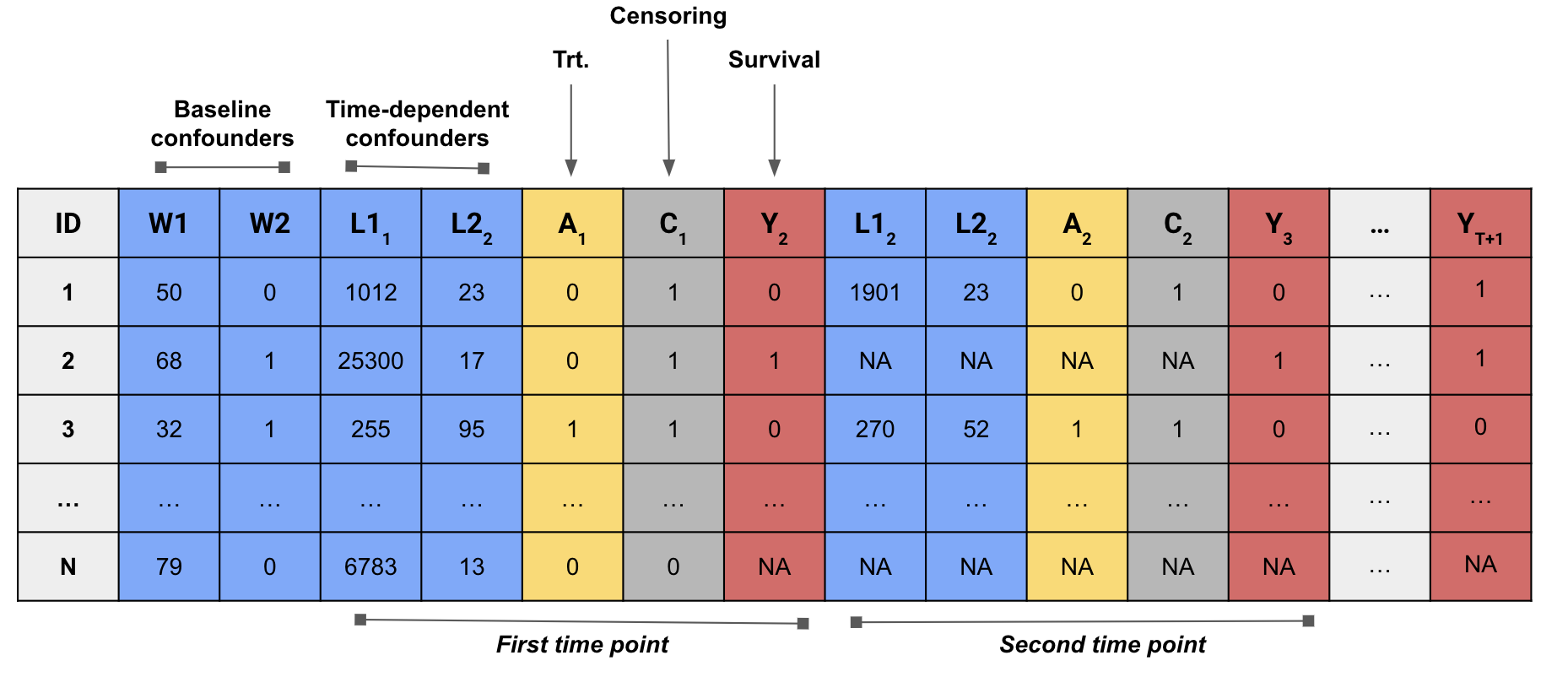
Data structure examples
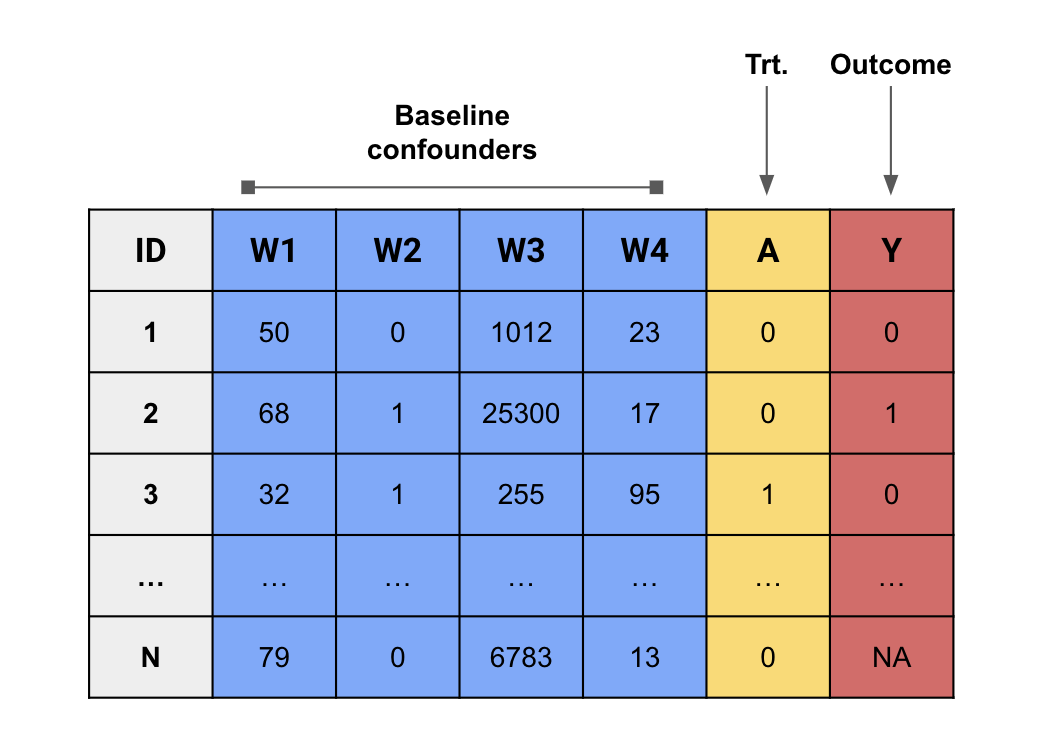
Point treatment
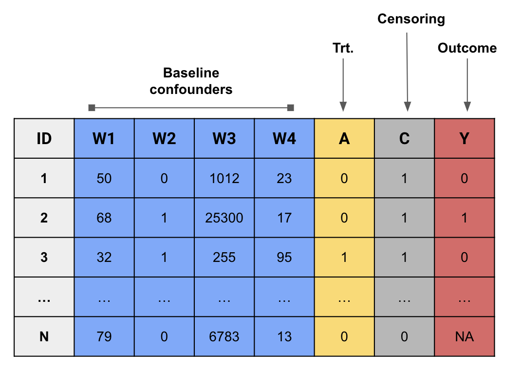
Point-treatment with censoring
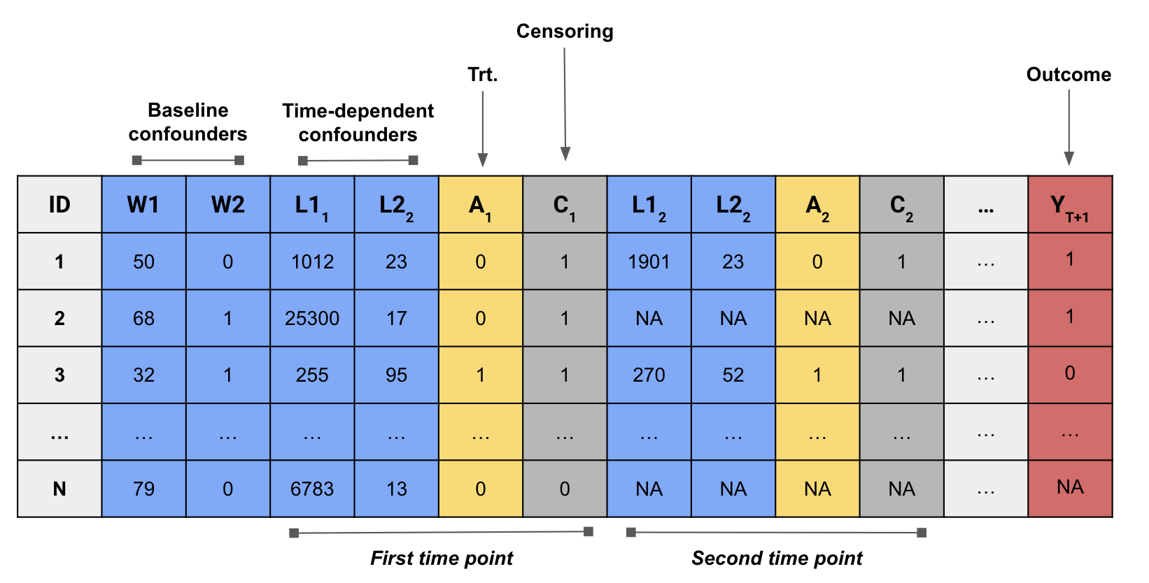
Time-varying treatment with censoring
Point-treatment with survival outcome
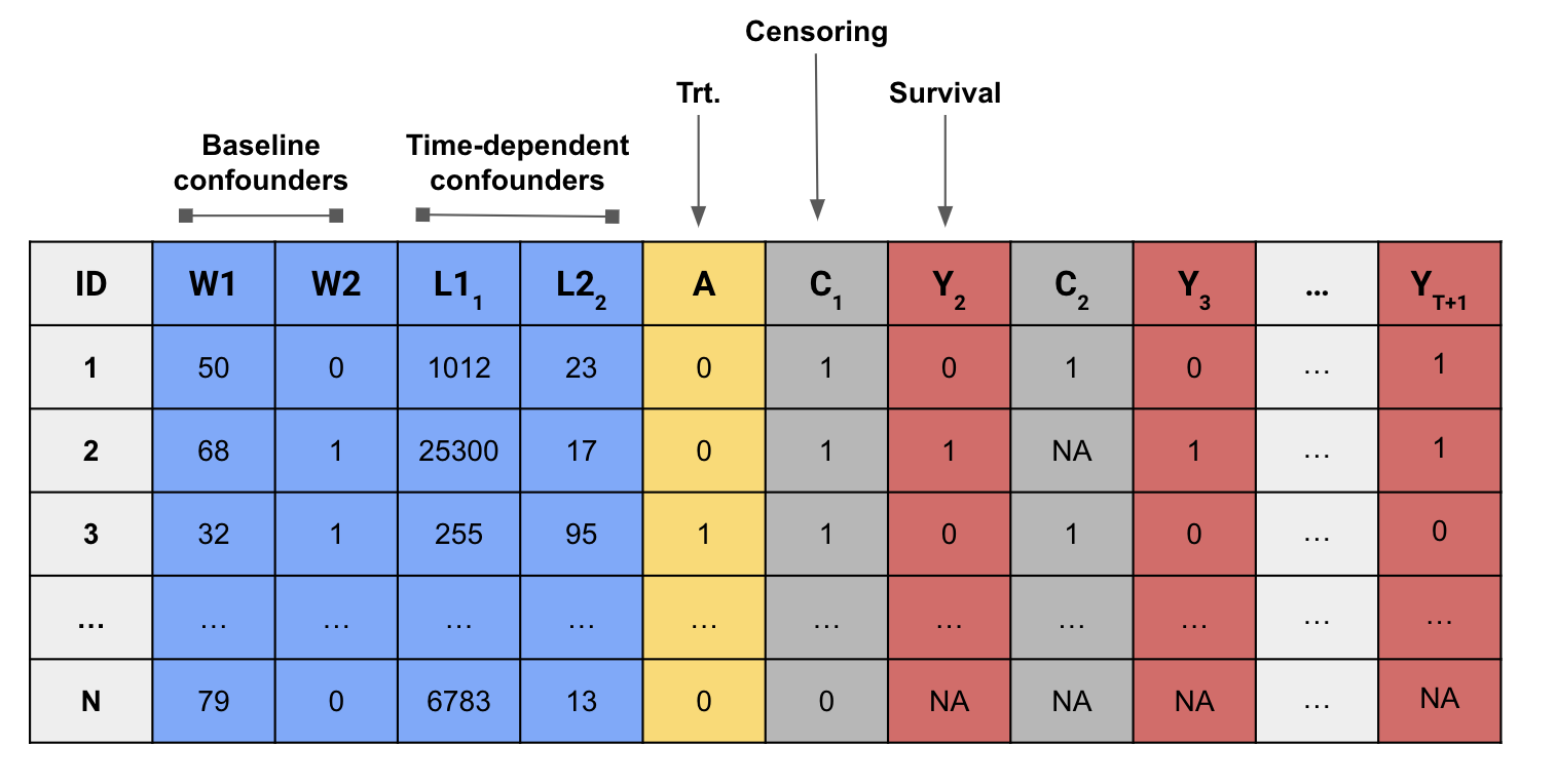
Time-varying treatment with survival outcome
Machine learning ensembles
As was already discussed, an attractive property of multiply-robust estimators is that they can incorporate flexible machine-learning algorithms for the estimation of nuisance parameters while remaining \(\sqrt{n}\)-consistent.
lmtp uses the super learner algorithm for estimating these nuisance parameters.
The super learner algorithm is an ensemble learner than incorporates a set of candidate models through a weighted convex-combination based on cross-validation. Asymptotically, this weighted combination of models, called the meta-learner, will outperform any single one of its components.
lmtp uses the implementation of the super learner provided by the
SuperLearnerpackage.The algorithms to be used in the super learner are specified with the
learners_trtandlearners_outcomearguments.The outcome variable type should guide users on selecting the appropriate candidate learners for use with the
learners_outcomeargument.Regardless of whether an exposure is continuous, dichotomous, or categorical, the exposure mechanism is estimated using classification. Therefore only include candidate learners capable of binary classification with the
learners_trtargument.Candidate learners that rely on cross-validation for the tuning of hyper-parameters should support grouped data if used with
learners_trt. Because estimation of the treatment mechanism relies on the augmented \(2n\) duplicated data set, duplicated observations must be put into the same fold during sample-splitting. This is done automatically by the package.
References
Dı́az, Iván, Nicholas Williams, Katherine L Hoffman, and Edward J Schenck. 2023. “Nonparametric Causal Effects Based on Longitudinal Modified Treatment Policies.” Journal of the American Statistical Association 118 (542): 846–57.
Van der Laan, Mark J, Eric C Polley, and Alan E Hubbard. 2007. “Super Learner.” Statistical Applications in Genetics and Molecular Biology 6 (1).
Williams, Nicholas, and Iván Dı́az. 2023. “Lmtp: An R Package for Estimating the Causal Effects of Modified Treatment Policies.” Observational Studies 9 (2): 103–22.